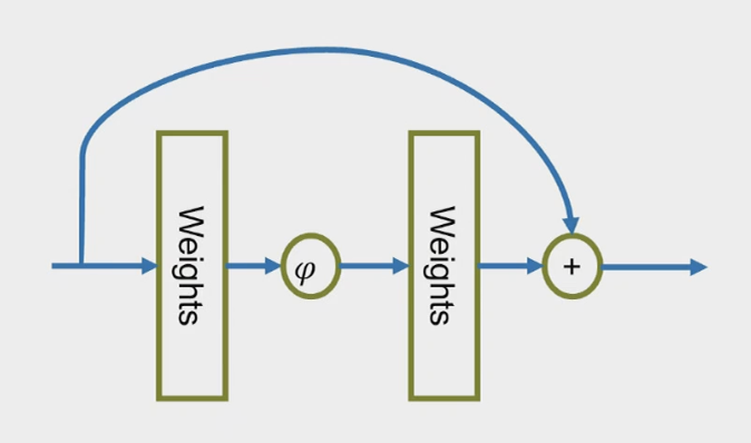
Support Vector Machines and the Maximum Margin Principle

This chapter is building up a really elegant story about how to choose the “best” linear classifier when your data is linearly separable — and then what to do when it isn’t. Let me walk you through it piece by piece.

The Core Problem: Too Many Perfect Classifiers

When data is linearly separable, there are infinitely many decision boundaries that correctly classify every training point. So which one should we pick? The chapter argues — convincingly — that we should pick the one that is maximally far away from the nearest data points on either side. This is the maximum margin classifier.

The intuition is simple: if your boundary has a wide “buffer zone” around it, then small perturbations to the data (or new test points drawn from a similar distribution) are less likely to end up on the wrong side.

Deriving the Distance Formula

To formalize “maximally far,” you need to measure the distance from a point to the decision boundary. The boundary is the set of points where ⟨w, x⟩ = 0 — a hyperplane through the origin.

Using the relationship between the dot product and the cosine of the angle between two vectors, the distance from a point x₀ to this hyperplane works out to |⟨w, x₀⟩| / ‖w‖₂. If you restrict w to have unit norm (‖w‖₂ = 1), the distance simplifies to just |⟨w, x₀⟩|. And since a correctly classified point satisfies y·⟨w, x⟩ > 0, you can drop the absolute value and write the signed distance as y·⟨w, x⟩.

The Margin and the Max-Margin Problem

The margin of a unit-norm classifier w is defined as the distance to the closest point in the training set:

$$\mathrm{margin}(w)=\underset{1\le i\le n}{\min }{y}_i⟨w,x_i⟩$$

The max-margin classifier $w_{\text{MM}}$ solves:

${\max }_{|w{|}_2=1}{\min }_{1\le i\le n}{y}_i⟨w,x_i⟩$

This is a minimax problem — maximize the worst-case distance. It’s conceptually clean but awkward to optimize directly.

The SVM Reformulation

Here’s where the SVM enters. Instead of maximizing the margin subject to unit norm, you flip the problem: minimize the norm of w subject to all points being at least distance 1 from the boundary:

${\min }_{w\in {\mathbb{R}}^d}|w{|}_2\text{s.t.}{y}_i⟨w,x_i⟩\ge 1\forall i$

Why is this equivalent? Think of it this way. The margin for a non-unit-norm w is min_i y_i⟨w, x_i⟩ / ‖w‖₂. The constraint y_i⟨w, x_i⟩ ≥ 1 forces the numerator to be at least 1, so the margin is at least 1/‖w‖₂. Minimizing ‖w‖₂ therefore maximizes 1/‖w‖₂, which maximizes the margin.

Lemma 8.1 formalizes this: w_SVM and w_MM point in the same direction — they differ only by a scalar. The proof works by showing that you can rescale w_MM to get a feasible solution to the SVM problem that achieves the same optimal norm, and since the SVM solution is unique, they must be the same (up to scale).

The support vectors are the training points that sit exactly on the margin boundary (where y_i⟨w, x_i⟩ = 1). These are the points “supporting” the decision boundary — if you removed any other point, the solution wouldn’t change.

Implicit Bias of Gradient Descent

This is a striking theoretical result. Suppose you don’t solve the SVM problem at all. Instead, you just run gradient descent on logistic loss — a smooth surrogate that never actually reaches zero on separable data. The iterates w_t will grow without bound in norm (the loss keeps getting pushed toward zero), so they never converge to a fixed point.

But Theorem 8.2 says their direction converges — and it converges exactly to w_MM, the max-margin classifier. Gradient descent on logistic loss “secretly” finds the SVM solution without you ever having to set up the constrained optimization problem. This is called the implicit bias of gradient descent: the algorithm’s own dynamics have a built-in preference for maximum margin, even though the loss function says nothing about margins.

When the data is not separable (Theorem 8.3), the story changes: the loss now has a unique finite minimizer, and gradient descent converges to it in the ordinary sense (not just in direction).

Soft-Margin SVM: Handling Non-Separable Data

For non-separable data, the hard constraint y_i⟨w, x_i⟩ ≥ 1 is impossible to satisfy for all points. The soft-margin SVM introduces slack variables ξ_i ≥ 0 that allow individual points to violate the margin:

${\min }_{w,\xi }\left(|w{|}_2^2+\lambda {\sum }_{i=1}^n{\xi }_i\right)\text{s.t.}{y}_i⟨w,x_i⟩\ge 1-{\xi }_i,;;{\xi }_i\ge 0$

Each ξ_i measures how much point i violates the margin. The parameter λ controls the trade-off: large λ penalizes violations heavily (approaching the hard-margin SVM if the data is separable), while small λ tolerates more violations and shrinks w toward zero.

The key insight at the end of the chapter is that you can eliminate the slack variables entirely. For a given w, the optimal ξ_i is just max(0, 1 − y_i w⊤x_i) — either the point satisfies the margin and ξ_i = 0, or it doesn’t and ξ_i equals the shortfall. Substituting this back gives the unconstrained form:

${\min }_w\left[|w{|}_2^2+\lambda {\sum }_{i=1}^n\max (0,1-y_i{w}^{\top }{x}_i)\right]$

The second term is the hinge loss. So the soft-margin SVM is really just ℓ₂ regularization plus hinge loss — a viewpoint that connects SVMs to the broader family of regularized empirical risk minimization methods you’ve likely seen elsewhere in the course.

---

The big picture takeaway: SVMs give you a principled way to select among all possible linear classifiers by maximizing the margin, this is equivalent to minimizing the norm of the weight vector, gradient descent on logistic loss finds this solution implicitly, and the soft-margin extension gracefully handles the non-separable case through the hinge loss.